Teaching a Single Neuron to Learn: Backpropagation and Gradient Descent in NumPy

In the previous post we built a single neuron and ran inputs through it. It worked, but there was a catch: we chose the weights 5, -1, and 0 ourselves. The neuron did not learn anything.

In this post we fix that. We will give the neuron random starting weights, show it examples with known answers, and let it work out the right weights by itself. The technique that makes this possible is backpropagation combined with gradient descent, and for a single neuron it fits in about ten lines of NumPy.

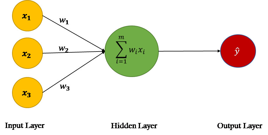
The big picture: how a neuron learns

Learning in a neural network follows the same four steps, over and over:

1. Forward pass: use the current weights to make a prediction.
2. Loss: measure how wrong the prediction is, as a single number.
3. Backward pass: work out how much each weight and the bias contributed to that error. These contributions are called gradients.
4. Update: nudge each weight a small step in the direction that reduces the error.

After enough repetitions, the weights settle somewhere that gives small errors. That is all "training" means.

Setting up a problem where we know the answer

To check that learning really works, we need to know what the right answer is. So we cheat in a useful way: we create a hidden "teacher" neuron with known weights, use it to produce the targets, and then see whether our student neuron can rediscover those weights from the data alone.

raw_inputs = np.array([
    [3, 1, 7],
    [4, 2, 5],
    [1, 0, 3],
    [6, 4, 2],
    [8, 5, 1],
    [2, 3, 9],
    [7, 7, 4],
    [0, 4, 6],
    [9, 1, 8],
    [5, 0, 8],
], dtype=float)
inputs = raw_inputs / 10

TRUE_WEIGHTS = np.array([4.0, -2.0, 0.0])
TRUE_BIAS = -1.0

def sigmoid(z):
    return 1 / (1 + np.exp(-z))

targets = sigmoid(inputs @ TRUE_WEIGHTS + TRUE_BIAS)  # each value is in (0, 1)

There are several things worth noticing here.

• The inputs are scaled down by 10. Raw values like 9 or 8 would make the weighted sum large, and sigmoid flattens out at large values, which makes learning very slow. Keeping inputs small and similar in size is a basic habit in machine learning.
• The teacher weights are [4, -2, 0] with bias -1. Same pattern as before: studying helps, partying hurts, and the third feature, shoe size, is irrelevant.
• Targets are probability-like numbers. Passing the teacher's weighted sum through sigmoid gives values between 0 and 1, for example 0.5 for the first row and 0.917 for the ninth.
• The student never sees the teacher's weights. It only sees the 10 input rows and their 10 target values.

The neuron, now with sigmoid and random weights

class SingleNeuron:
    def __init__(self, n_inputs: int, seed=42, learning_rate=0.5) -> None:
        rng = np.random.default_rng(seed)
        self.weights = rng.random(n_inputs)  # random start: nowhere near the truth
        self.bias = 0.0
        self.learning_rate = learning_rate

Compared to the first post, there are three changes:

• The weights start as random numbers between 0 and 1, produced by NumPy's random generator. The seed=42 makes the "random" numbers the same on every run, so your results match the ones in this post.
• The bias starts at 0.
• There is a new learning_rate, which controls how big each update step is. We will come back to it.

We also drop the choice of activation and use sigmoid only. The reason is that learning needs a smooth function we can take derivatives of, and sigmoid is both smooth and gives outputs in the same (0, 1) range as our targets.

    def forward(self, single_input: np.ndarray) -> float:
        forward_measure = np.dot(single_input, self.weights) + self.bias
        return self.activation_function(forward_measure)

    def activation_function(self, forward_measure: float) -> float:
        return sigmoid(forward_measure)

The forward pass is unchanged. The random starting weights are [0.774, 0.439, 0.859], which are nowhere near the true [4, -2, 0], so the early predictions are poor.

Step 2: the loss function

To improve, the neuron needs a number that says how bad its prediction is. We use half the squared difference between the target and the prediction:

    def loss(self, predicted_value: float, target_value: float):
        return 1 / 2 * (target_value - predicted_value) ** 2

• If the prediction equals the target, the loss is 0.
• Squaring makes every error positive, so being too high and too low both count as bad.
• Squaring also punishes big errors much more than small ones.
• The factor of 1/2 is there for convenience: when we take the derivative, the 2 from the square cancels it.

This is called the squared error or mean squared error loss (it is a mean when averaged over many examples). The goal of training is to make this number as small as possible.

Step 3: the backward pass

Now the key question: if we want to lower the loss, should we make each weight bigger or smaller, and by how much?

The answer is the gradient, the derivative of the loss with respect to each weight. It tells us how sensitive the loss is to that weight. A positive gradient means increasing the weight would increase the loss, so we should decrease it. A negative gradient means the opposite.

The chain of calculations

The loss depends on the weights through a chain of three steps:

z = w1*x1 + w2*x2 + w3*x3 + b      (weighted sum)
p = sigmoid(z)                      (prediction)
L = 1/2 * (t - p)^2                 (loss)

A weight affects z, z affects p, and p affects L. To find how L changes when a weight changes, we multiply the derivatives of each link. This is the chain rule from calculus:

dL/dw_i = dL/dp * dp/dz * dz/dw_i
dL/db   = dL/dp * dp/dz * dz/db

Each piece is simple on its own:

dL/dp    = (p - t)          derivative of 1/2 * (t - p)^2 with respect to p
dp/dz    = p * (1 - p)      derivative of sigmoid
dz/dw_i  = x_i              only the term w_i * x_i contains w_i
dz/db    = 1                b is simply added

The derivative of sigmoid has a neat form: if p = sigmoid(z), then the slope is p * (1 - p). That means we can compute it from the prediction we already have, without calling sigmoid again.

Multiplying the pieces together gives exactly the two formulas in the code:

dL/dw_i = (p - t) * p * (1 - p) * x_i
dL/db   = (p - t) * p * (1 - p)

    def dL_dw(self, predicted_value: float, target_value: float, input_value: float):
        return (predicted_value - target_value) * predicted_value * (1 - predicted_value) * input_value

    def dL_db(self, predicted_value: float, target_value: float):
        return (predicted_value - target_value) * predicted_value * (1 - predicted_value)

Notice the repeated part (p - t) * p * (1 - p). It is the same in both methods, and the weight gradient just multiplies it by the input x_i. This makes intuitive sense:

• An input that is large has more influence on z, so its weight gets a bigger gradient.
• An input that is 0 gets a gradient of exactly 0, so its weight is never changed by that example.
• The bias is like a weight whose input is always 1, so it gets the shared part without any multiplier.

The name "backpropagation" comes from this: we start from the loss at the end and propagate the error backward through the chain, toward the weights. With one neuron the chain is short. In later posts, with many layers, the same idea reuses these pieces again and again.

Step 4: the update (gradient descent)

    def backward_pass(self, single_input: np.ndarray, predicted_value: float, target_value: float):
        # Update the weights
        for i, w in enumerate(self.weights):
            self.weights[i] = w - self.learning_rate * self.dL_dw(
                predicted_value=predicted_value, target_value=target_value, input_value=single_input[i])

        # Update the bias
        self.bias = self.bias - self.learning_rate * self.dL_db(
            predicted_value=predicted_value, target_value=target_value)

Each weight is updated with the same rule:

new_weight = old_weight - learning_rate * gradient

We subtract the gradient because the gradient points uphill, in the direction where the loss grows. Subtracting moves us downhill. This method of repeatedly stepping downhill is called gradient descent.

The learning rate scales the step. If it is too large, the weights can overshoot and bounce around or even diverge. If it is too small, learning crawls. A value of 0.5 works well for this tiny problem, but there is no universal best value, and it is one of the first things to tune in a real project.

One detail about the code: the loop reads the prediction predicted_value that was calculated before any update. Since all the gradients are based on the same prediction, the order in which we update the weights does not matter.

One update, by hand

Let's follow a single training step with the first row, using the random starting weights, so you can see that nothing mysterious happens:

x       = [0.3, 0.1, 0.7]          (the first row, divided by 10)
weights = [0.774, 0.439, 0.859]    (random start), bias = 0.0
target  = 0.500

z    = 0.3*0.774 + 0.1*0.439 + 0.7*0.859 + 0.0 = 0.877
p    = sigmoid(0.877)                          = 0.706
loss = 1/2 * (0.5 - 0.706)^2                   = 0.0213

delta = (p - t) * p * (1 - p)
      = (0.706 - 0.5) * 0.706 * 0.294          = 0.0428

grad w1 = 0.0428 * 0.3 = 0.0128
grad w2 = 0.0428 * 0.1 = 0.0043
grad w3 = 0.0428 * 0.7 = 0.0299
grad b  = 0.0428

w1 = 0.774 - 0.5 * 0.0128 = 0.768
w2 = 0.439 - 0.5 * 0.0043 = 0.437
w3 = 0.859 - 0.5 * 0.0299 = 0.844
b  = 0.0   - 0.5 * 0.0428 = -0.021

The prediction moves from 0.706 to 0.699, a little closer to the target of 0.5, and the loss drops from 0.0213 to 0.0198. One step does very little. But training does thousands of these steps, and they add up.

The training loop

Putting the pieces together:

nn = SingleNeuron(n_inputs=3, learning_rate=0.5)

for epoch in range(500):
    total_loss = 0.0
    for x_i, target_value in zip(inputs, targets):
        predicted_value = nn.forward(x_i)                       # 1. forward
        total_loss += nn.loss(predicted_value, target_value)    # 2. measure the error
        nn.backward_pass(x_i, predicted_value, target_value)    # 3. backward + update

• One pass through all the examples is an epoch. We run 500 epochs.
• Within an epoch, we update the weights after every single example. This is called stochastic gradient descent (SGD) in its simplest form. Other versions average the gradient over many examples before updating, and we will meet them later.
• total_loss adds up the loss over the epoch, so dividing by the number of examples gives the average loss that we print.

The full code

import numpy as np

raw_inputs = np.array([
    [3, 1, 7],
    [4, 2, 5],
    [1, 0, 3],
    [6, 4, 2],
    [8, 5, 1],
    [2, 3, 9],
    [7, 7, 4],
    [0, 4, 6],
    [9, 1, 8],
    [5, 0, 8],
], dtype=float)
inputs = raw_inputs / 10

TRUE_WEIGHTS = np.array([4.0, -2.0, 0.0])
TRUE_BIAS = -1.0

def sigmoid(z):
    return 1 / (1 + np.exp(-z))

targets = sigmoid(inputs @ TRUE_WEIGHTS + TRUE_BIAS)  # each value is in (0, 1)

class SingleNeuron:
    def __init__(self, n_inputs: int, seed=42, learning_rate=0.5) -> None:
        rng = np.random.default_rng(seed)
        self.weights = rng.random(n_inputs)  # random start: nowhere near the truth
        self.bias = 0.0
        self.learning_rate = learning_rate

    def forward(self, single_input: np.ndarray) -> float:
        forward_measure = np.dot(single_input, self.weights) + self.bias
        return self.activation_function(forward_measure)

    def activation_function(self, forward_measure: float) -> float:
        return sigmoid(forward_measure)

    def loss(self, predicted_value: float, target_value: float):
        return 1 / 2 * (target_value - predicted_value) ** 2

    def dL_dw(self, predicted_value: float, target_value: float, input_value: float):
        return (predicted_value - target_value) * predicted_value * (1 - predicted_value) * input_value

    def dL_db(self, predicted_value: float, target_value: float):
        return (predicted_value - target_value) * predicted_value * (1 - predicted_value)

    def backward_pass(self, single_input: np.ndarray, predicted_value: float, target_value: float):
        # Update the weights
        for i, w in enumerate(self.weights):
            self.weights[i] = w - self.learning_rate * self.dL_dw(
                predicted_value=predicted_value, target_value=target_value, input_value=single_input[i])

        # Update the bias
        self.bias = self.bias - self.learning_rate * self.dL_db(
            predicted_value=predicted_value, target_value=target_value)


if __name__ == "__main__":
    nn = SingleNeuron(n_inputs=3, learning_rate=0.5)

    print("True weights :", TRUE_WEIGHTS, "| true bias:", TRUE_BIAS)
    print("Start weights:", nn.weights.round(3), "| start bias:", nn.bias)
    print()

    for epoch in range(500):
        total_loss = 0.0
        for x_i, target_value in zip(inputs, targets):
            predicted_value = nn.forward(x_i)
            total_loss += nn.loss(predicted_value, target_value)
            nn.backward_pass(x_i, predicted_value, target_value)

        if epoch % 50 == 0:
            print(f"epoch {epoch:4d} | avg loss {total_loss / len(inputs):.2e} | "
                  f"weights {nn.weights.round(3)} | bias {nn.bias:.3f}")

    print()
    print("Learned weights:", nn.weights.round(3), "| learned bias:", round(nn.bias, 3))
    print("True weights   :", TRUE_WEIGHTS, "| true bias   :", TRUE_BIAS)

What the neuron learned

Running the program prints this (I print every 50 epochs here, so we can watch the progress):

True weights : [ 4. -2.  0.] | true bias: -1.0
Start weights: [0.774 0.439 0.859] | start bias: 0.0

epoch    0 | avg loss 2.85e-02 | weights [0.76  0.393 0.766] | bias -0.152
epoch   50 | avg loss 4.40e-03 | weights [ 2.227 -0.243  0.134] | bias -0.774
epoch  100 | avg loss 1.81e-03 | weights [ 2.837 -0.704  0.059] | bias -0.881
epoch  150 | avg loss 8.96e-04 | weights [ 3.162 -1.036  0.042] | bias -0.925
epoch  200 | avg loss 4.83e-04 | weights [ 3.368 -1.274  0.033] | bias -0.945
epoch  250 | avg loss 2.74e-04 | weights [ 3.513 -1.446  0.024] | bias -0.957
epoch  300 | avg loss 1.60e-04 | weights [ 3.619 -1.573  0.017] | bias -0.964
epoch  350 | avg loss 9.59e-05 | weights [ 3.7   -1.668  0.011] | bias -0.969
epoch  400 | avg loss 5.85e-05 | weights [ 3.762 -1.74   0.006] | bias -0.973
epoch  450 | avg loss 3.61e-05 | weights [ 3.810e+00 -1.796e+00  3.000e-03] | bias -0.976

Learned weights: [ 3.847e+00 -1.838e+00  1.000e-03] | learned bias: -0.979
True weights   : [ 4. -2.  0.] | true bias   : -1.0

There is a lot to see here:

• The loss falls steadily, from about 0.0285 in the first epoch to about 0.00004 after 450. The error shrank by a factor of several hundred.
• The weights move toward the true ones. The first weight climbs from 0.77 toward 4, and the second goes from positive 0.44 to negative 1.84, heading toward -2. The neuron discovered on its own that partying lowers the output.
• The shoe size weight shrinks toward zero. It started at 0.859, the largest of the three. Since shoe size has no real effect on the target, the gradients keep pushing it down, and it ends at about 0.001. The neuron learned to ignore an irrelevant feature, without being told.
• The bias heads to -1. It ends at about -0.979.

Why aren't the learned values exactly 4, -2, 0, and -1?

They are close but not exact, and the log shows why: the loss is still decreasing at epoch 500. Learning slows down as it nears the answer, because the gradient gets smaller when the error does. Two other things add to the slowness:

• The sigmoid slope p * (1 - p) is never larger than 0.25, which shrinks every gradient.
• The inputs are small (0 to 0.9), which also shrinks the weight gradients.

Training for more epochs would get closer still. For practical purposes, the neuron already predicts the targets very well: for the first row, the target is 0.5000 and the trained neuron predicts 0.4978.

Note also that the weights are not the only way to match the data. When only 10 examples are available, several slightly different weight combinations can give nearly the same predictions. Here the data is clean and was made by a neuron of the same shape, so the answer is recoverable, but with real data you rarely have that guarantee.

Common things to try

1. Change the learning rate to 0.05 and then to 5. Watch the loss: at 0.05 it learns much more slowly, and at 5 it may become unstable.
2. Change the seed and see that different starting points still end up at similar weights.
3. Remove the division by 10 and see how much harder it becomes for the neuron to learn.
4. Run more epochs and watch the weights get closer to [4, -2, 0] and the bias to -1.

Key takeaways

1. Learning means finding weights that make the loss small, by repeating forward pass, loss, backward pass, and update.
2. The loss turns "how wrong are we?" into one number. Here it is half the squared error.
3. The gradient says how the loss changes when a weight changes. The chain rule gives it as (p - t) * p * (1 - p) * x for weights and the same without x for the bias.
4. Gradient descent subtracts the gradient times the learning rate, so each step moves downhill.
5. Irrelevant inputs end up with weights near zero, and useful ones grow in the right direction.

What's next

Our neuron can learn, but the code is slow and clumsy: loops over examples and over weights. In the next post we will replace those loops with vectorized NumPy operations, so the whole dataset can be processed at once. After that we will connect several neurons into a layer, which is the first step toward a real neural network.